Financial forecasting is crucial for any organisation but can be especially challenging for hospitals. Many factors contribute to the complexity of predicting future financial performance. This is where accounting and forecasting solutions offer a powerful tool to navigate uncertainties and make data-driven decisions.

This article explores an innovative accounting forecasting solution designed specifically to forecast a hospital group's monthly revenue and expenses comprising various hospitals from different locations and departments within each hospital.

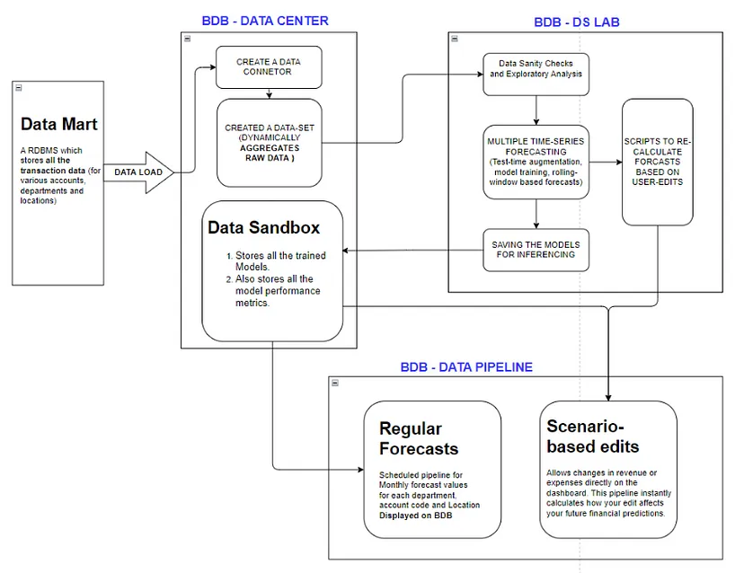
We’ll delve into its architecture, highlighting how it leverages historical data, time-series regression approach, and scenario planning to provide valuable insights for financial planning and budgeting for each department across different hospitals. The solution implementation diagram is provided below.

Building the Foundation: Data Acquisition and Transformations

The solution efficiently extracts raw data from a community health system, including expenses, revenues, locations, accounts, and departments. This system encompasses pharmacies and clinics. With accounting calculations meticulously performed under the guidance of a subject matter expert, the resulting dataset, augmented with accurately calculated accounting figures, serves as the cornerstone for the forecasting process.

After performing the above-mentioned process, the cleaned (almost) data is added to a data mart. This specialised data storage is a central hub that organizes and processes the extracted structured data. We store each transaction line item in the data mart before loading it into the BDB-Decision Platform platform again for further aggregations and processing.

The platform is where the final training data is made. Here, the calculated data undergoes transformations, getting aggregated on a monthly basis for the past 20 years. This historical depth provides a rich understanding of trends and patterns for the modelling process. It is crucial for making informed future predictions.

The forecasting process is conducted for each department across different hospital locations, ensuring a comprehensive analysis of financial trends and performance metrics. We will discuss the forecasting process in more depth below.

Granular Forecasting with Machine Learning

Dataset overview

At this stage, the data looks like a multiple-time series problem; every location, department and sub-departments have their own time series. There is, of course, the aggregated overall time series information for each location, department or hospital group as a whole (all locations).

The solution takes a granular approach to forecasting. It utilizes machine learning to train multiple independent models for this multiple time-series data set. Each model focuses on a specific department, location, and sub-department combination. After loading the data in the DS-Lab module, we clean it and imputation it. Then we run some statistical tests to check data sanity and feasibility for training an accurate time series model. Then, this data set undergoes an exhaustive feature engineering process that combines various lags, moving averages, and principal component analysis to extract the best features for model training. The model approach and feature engineering are described in more detail below.

Modelling Approach

We have focused on time-series-specific feature engineering. The feature engineering process includes a combination of the following:

• Autoregressive elements: creating lag variables.
• Aggregated features on lagged variables: moving averages, exponential smoothing descriptive statistics, correlations.
• Date-specific features: week number, day of week, month, year.
• Target transformations: Integration/Differentiation, univariate transforms (like logs, square roots)
• Principal component Analysis: combining different features

These feature transforms are applied to each time-series model that we have trained. Tree-based gradient boosting models perform the best for our data. We perform a 5-fold Time Series cross-validation to select the best hyperparameters.

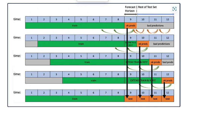
Rolling-Window-Based Predictions

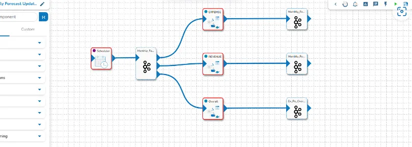
Once we have the models trained in DS-Lab, we save them for inferencing on demand. We use Test-Time Augmentation for future predictions. It helps assess the performance of the pipeline for predicting not just a single forecast horizon but many in succession. TTA simulates the process where the model stays the same, but the features are refreshed using newly available data. Once new data is available(every month), a scheduler is triggered, which initiates the re-fitting of the entire pipeline on the newly available data. This monthly run pipeline retrains the existing models on the updated data. After that, we used Test-Time augmentation for Downstream Impact Analysis to understand the Ripple Effect of different simulated financial events and scenarios on the current forecasts. This is discussed in the section below.

Model maintenance and retraining

These models are not static entities. They are trained monthly through a scheduled pipeline, constantly adapting to evolving trends and hospital dynamics. This ongoing learning process guarantees the accuracy and reliability of the forecasts. A pipeline updates the data mart to access the data as soon as new data is updated in the raw data sets. This change in the underlying data mart triggers the retraining pipeline.

But the solution goes beyond mere prediction. It tracks every model’s performance, records accuracy metrics, and filters poor-performance models. This comprehensive data allows continuous improvement and ensures the models remain optimized over time.

Downstream Impact Analysis: Understanding the Ripple Effect

Forecasting isn’t just about predicting the future; it’s about understanding the consequences of present actions. This solution offers a unique feature — downstream impact analysis. Imagine you’re reviewing the financial dashboard and deciding to adjust a specific expense value based on your business knowledge and intuition. With this feature, you can witness the ripple effect of this change on all downstream forecasts for that series. The forecasting model is broadly divided into two categories: the overall forecast models and the granular forecast models. The overall forecasting models take care of accurate predictions for overall expense and revenue across all locations. In contrast, the granular forecasting models forecast expense/revenue for each account code, department and location.

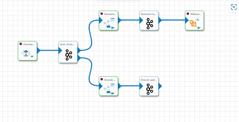
We have made a separate pipeline for doing the scenario-based downstream calculations. An API ingestion component is waiting at the head of the pipeline for a trigger from the dashboard after an edit by the user, we capture these scenarios, make features and forecast them accordingly. We also capture the difference in actual value and assumption the user made to trigger the overall model and update the graphs in the Dashboard. It can be seen in the second arm of the data pipeline, which handles updating and triggering the overall forecasts based on user edits, even on the granular time-series.

The secret lies in the saved models. These models capture the intricate relationships between different financial elements within the hospital. By triggering an API ingestion component, the solution can load the relevant model and recalculate the downstream forecasts based on the edited value. This allows you to explore various scenarios and make informed decisions with a clear picture of potential consequences. The overall solution diagram and its implementation is shown below:

Creating different versions of these scenarios further enhances the solution’s versatility. You can explore the impact of changes under various assumptions, empowering you to navigate complex financial landscapes with greater confidence and solutions in the BDB-Decision Platform.